Calculation of a Delaunay triangulation
Release 1.0
2026 October
This article describes how to compute Delaunay triangulations using algorithms ranging from the simplest to the most complex and high-performance ones.
The final method presented highlights an innovative approach suitable for large datasets.
The algorithms presented are evaluated using several datasets derived from topographic surveys.
The evaluations rely on metrics to assess algorithm complexity, computational load, and memory usage.
This article is available in PDF format.
- Delaunay triangulation
- Topological model of triangulations
- Inserting an interior vertex
- Inserting a vertex on a segment
- Shift the adjacent side of two triangles
- Delaunay criterion for two adjacent triangles
- Base max and height of a triangle
- The relative axis tool
- Status of a point
- Base criterion for two adjacent triangles
- OOP implementation of the topological model
- Evaluation metrics
- Sample test dataset
- Bowyer–Watson algorithm the reference
- Flip algorithm
- Optimization via tree-based sorting
- Algorithm with convex hull
- Convex ring algorithm
- Evaluation with other datasets
- Assessment of method complexity
- Evaluating the strengths and weaknesses of the methods
- General conclusion
- References
Delaunay triangulation
Boris Delaunay was a Russian mathematician born in 1890, well known for Delaunay triangulation (1934).
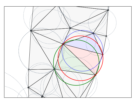
The Delaunay triangulation of a set of points in the plane subdivides the space into triangles whose circumcircles contain none of the points.
|
This method maximizes the size of the smallest angle among all the triangles and tends to avoid skinny triangles. This method is used in numerous fields of application, notably surveying, to calculate the contour lines of a terrain based on a network of points with measured elevations. The illustration highlights three adjacent triangles (red, green, blue) that satisfy the Delaunay criterion, along with their circumcircles. |
Topological model of triangulations
The topological model of a triangulation allows for navigation from triangle to triangle and the performance of operations on the triangles while maintaining the consistency of the network.
|
Each triangle in the mesh references its three vertices (S Up to three triangles (T
|
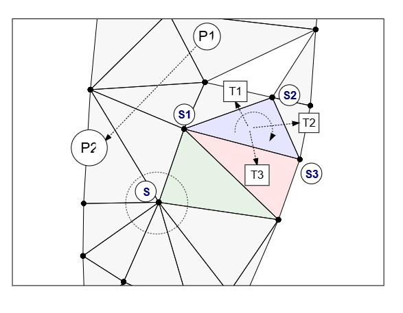
In principle, all triangles are described in the same direction of rotation. For convenience, clockwise, so as to obtain a positive area:
area(S1,S2,S3) = (x2-x1)*(y1+y2)/2+(x3-x2)*(y2+y3)/2+(x1-x3)*(y3+y1)/2
This also simplifies the (strict) inclusion test for a point p(x,y) within the triangle (S1,S2,S3) by determining the three areas (S1,S2,p), (S2,S3,p), and (S3,S1,p), all of which must be strictly positive:
area(S1,S2,p) > 0 and area(S2,S3,p) > 0 and area(S3,S1,p) > 0
The topological model of the triangulation supports several operations, such as:
Inserting an interior vertex
This operation completes the triangulation by subdividing a triangle into three, using a new vertex strictly inside the triangle.
For convenience, this operation is referred to as "split triangle" in the remainder of this document, denoting the division of a triangle into three by inserting a point inside.
|
| ||||||||||||||||||||||||||||||||||||||||||
Before inserting vertex Vi into triangle Ta | After inserting vertex Vi into triangle Ta | ||||||||||||||||||||||||||||||||||||||||||
|
|
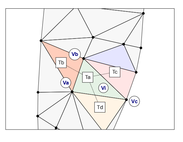
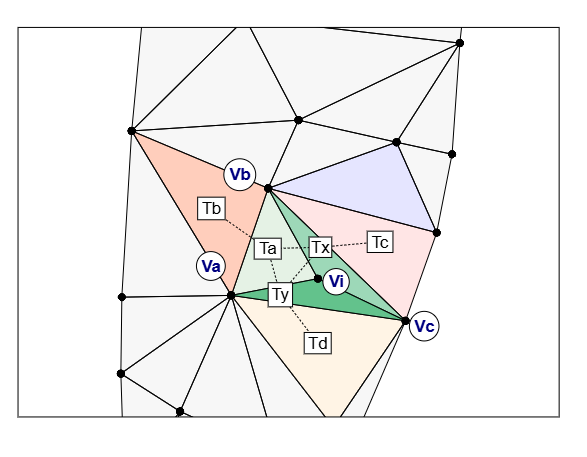
The operation modifies triangle Ta and inserts the two triangles (Tx,Ty).
Inserting a vertex on a segment
This operation completes the triangulation by inserting a vertex on the edge of a triangle, thereby subdividing that triangle into two, as well as the adjacent triangle sharing that edge, if one is defined.
For convenience, this operation is referred to as "split segment" in the remainder of this document, denoting the division of two triangles into four by inserting a point on the shared segment.
|
| ||||||||||||||||||||||||||||||||||||||||||||||||||||||||
Before inserting vertex Vi onto the segment (Vb, Vc)
|
After inserting vertex Vi onto the segment (Vb, Vc)
| ||||||||||||||||||||||||||||||||||||||||||||||||||||||||
|
|
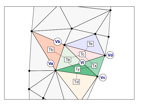
The operation modifies triangles (Ta,Tc) and inserts the two triangles (Tx,Ty).
Shift the adjacent side of two triangles
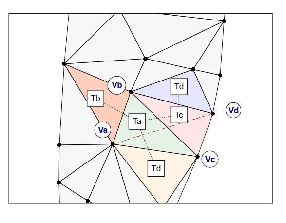
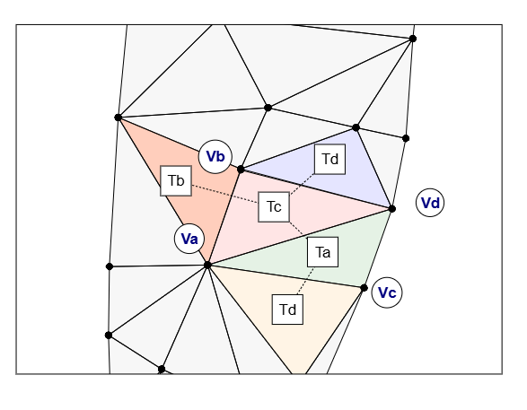
This operation transforms two adjacent triangles by flipping the vertices of their shared side onto the opposite vertices.
Transformation of triangles (T by flipping the common edge a,Tc)(V to b, Vc)(V:
a, Vd)
|
| ||||||||||||||||||||||||||||||||||||||||||
| Before transformation | After transformation | ||||||||||||||||||||||||||||||||||||||||||
|
|
Delaunay criterion for two adjacent triangles
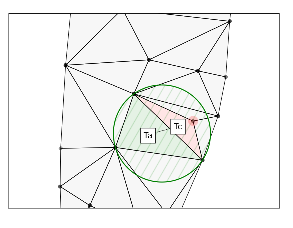
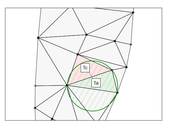
Two adjacent triangles do not satisfy the Delaunay condition if one of the two vertices opposite the shared edge lies within the circumcircle of the triangle formed by the other vertex.
|
| ||
|
The vertex of
The two triangles |
After the shift transformation the two triangles meet the criterion. |
Base max and height of a triangle
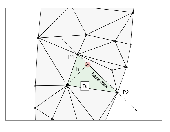
The maximum base of a triangle is its longest side, with the opposite vertex situated orthogonally to it.
|
Measure the height from the longest base to the opposite vertex, and finally, the height-to-base-length ratio.
To determine the maximum base, the relative axis measurement tool (P |
The relative axis tool
The relative axis is to geometric calculation what the ruler and set square are to technical drawing. That is, an indispensable tool.
|
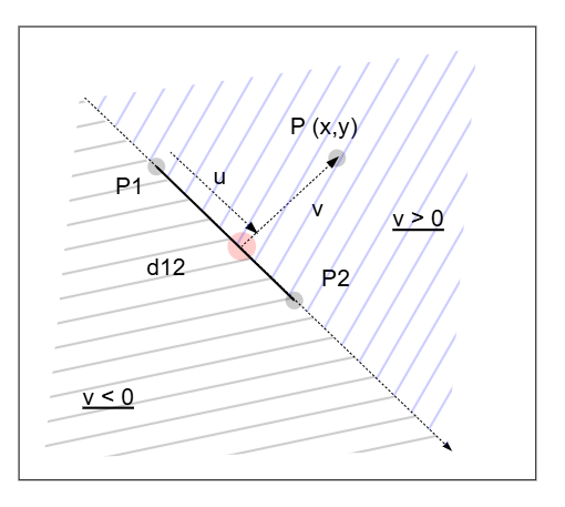
The relative axis, defined by two points (P
The value t, equal to u divided by the distance d12 between P The axis divides the space into two sectors (positive v, negative v). |
Examples of using the relative axis to calculate a triangle's circumcircle and its distance to a point.
|
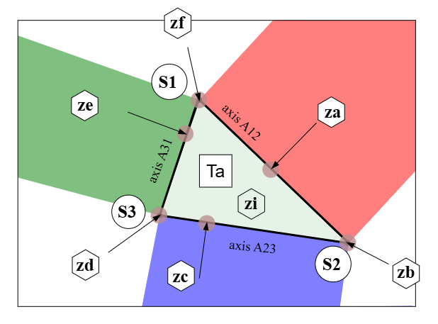
The circumcenter of triangle Ta is determined by the intersection of the perpendicular bisectors (A |
Calculation of the distance from a point to the triangle, the axes of the 3 sides divide the space into 7 zones:
|
|
Status of a point
The triangulation incorporates the computational precision required to handle edge cases, such as point-to-point or point-to-segment proximity.
A point's position relative to a triangle is characterized by a status.
|
The status is an enumeration used to distinguish between cases, the radius represents the calculation precision of the triangulation:
|
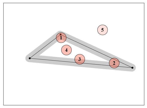
Determining point status significantly impacts triangulation calculation methods, particularly when handling edge cases in operations such as inserting a point inside a triangle or onto a segment.
In particular, points with "near vertex" status are excluded from the triangulation, listed, and flagged as a dataset anomaly.
Base criterion for two adjacent triangles
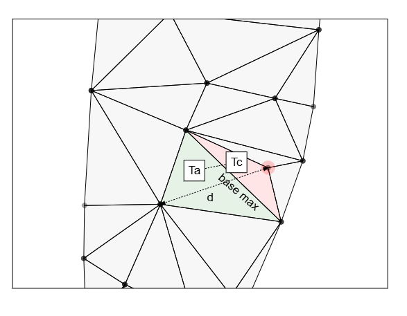
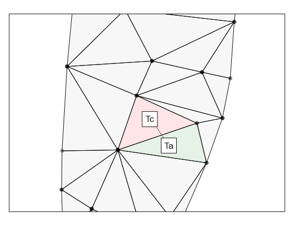
Two triangles sharing a common base max, with the distance between their opposite vertices being less than the length of the common base, are candidates for transformation by swapping the common base with the edge connecting their opposite vertices.
This criterion makes it possible to improve triangle quality without calculating circumcircles. It can be used prior to Delaunay criteria.
|
|
OOP implementation of the topological model
An object-oriented implementation (OOP) of the triangulation's topological model establishes a logical foundation that enables the development of various methods.
The kernel consists of three classes of objects:
Vertex
It may be identical to the dataset's point class, or constitute an enriched class containing a link to a triangle built on that vertex, serving as an entry point into the triangulation.
Provides its (x, y) coordinates.
Triangle
Class holding links to its 3 vertices and its one to three adjacent triangles.
Its public methods are read-only for the object.
Triangulation
Class that holds the triangles and contains the logic for creating and transforming them.
All the methods described in this document are based on this model.
Evaluation metrics
To compare methods, several indicators are measured:
Duration (Ms), the execution time (indicative) in milliseconds
This metric is provided for informational purposes; due to the execution platform (Desktop Intel Core i5 32Go,Windows 11/Java), it may vary from one execution to another.
Memory (Kb), the amount of memory in kilobytes.
This measure is calculated by summing the sizes of the objects' data members.
Classes, the number of OOP classes.
Only application classes are counted. Technical classes, such as lists, are not included in the count.
Objects, the number of allocated objects.
Triangle, the number of created triangles.
Conformity (C. %), the Delaunay conformity of the triangulation in percentage after point insertion step.
Distance the number of distance calculations in thousands.
Only distances calculated between points.
Axis tool, the number of axis calculations in thousands.
Point status (P. status), the number of point status calculations in thousands.
Circle, the number of circumcircle calculations in thousands
Insert, the number of triangle point insertion
Split segment, the number of segment point insertion
Shift, the number of triangle transformations resulting from the application of the Delaunay criterion and the base-max criterion.
Scan (Sc.), the number of full scans of the triangulation triangles.
Near vertex status (N. v, the number of points with "near vertex" status excluded from the triangulation.
Near segment status (N. s), the number of cases with "near segment" or "near angular sector"status.
This two last metrics characterizes the quality of the dataset.
Op (Σ op), the total number of geometric operations counted (distance, axis, P. status, circle) in thousands.
Axis and circle: counts only the number of constructed objects and encompasses all method calls on those objects.
Distance: only distances calculated between points; metrics distinct from axis and circle.
Σ pt the total number of geometric operations per point.
B. p the amount of memory in bytes per point.
Ratio calculated as the number of operations per point of the reference method DtRef divided by that of the method under consideration.
Provides a comparison criterion that is inversely related to the method's computational load.
Sample test dataset
The calculation methods presented below are illustrated using a sample of real points. This consists of a topographic survey of leveling points.
The sample consists of 981 points covering an area of 9,700 x 6,300 meters. The calculation precision is set to 1 centimeter.
The non-convex perimeter is irregular because it borders rivers.
 |
The distribution of the points is not random as shown in the illustration below, but proceeds step-by-step following the operators' movements in the field.
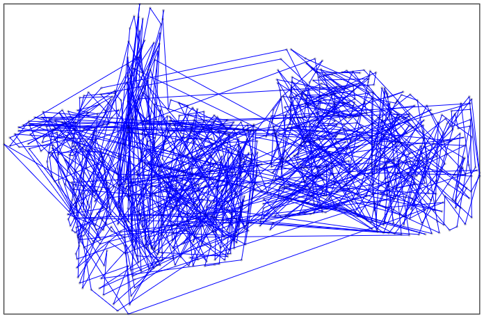 |
This property is important for the subsequent calculations.
Bowyer–Watson algorithm the reference
The Bowyer-Watson algorithm is an iterative algorithm.
It proceeds by adding points, one at a time, to a valid Delaunay triangulation of the subset of points. After each insertion, all triangles whose circumcircle contains the new point are removed, leaving a convex polygonal hole that is then re-triangulated using the new point.
The triangulation is initialized with a fictitious "super-triangle" enclosing all the points by adding specific points, which can be constructed as follows:
Determine the bounding box of the points (center (xc, yc), width, height)
Set the radius r = Max(width, height) / 2, this value can be increased to move away from the limit points.
Set p1 = (xc, yc + 2*r)
Set p2 = (xc + 3*r, yc - r)
Set p3 = (xc - 3*r, yc - r)
After creating the triangulation, the triangles located along the edges of the fictitious envelope must be removed.
Finally, the triangulation boundary may extend beyond the actual perimeter of the point set, resulting in triangles with abnormal lengths (or ratios). In such cases, the boundary must be reduced by removing the abnormal triangles along the edges.
The Bowyer–Watson algorithm can be summarized as follows:
1/ Create the "super triangle"
2/ Insert the scatter points
    For each point (p):
    - find the triangle (t) containing point (p)
    - remove the triangles adjacent to (t) whose circumcircle contains the new point (p)
    - triangulate the polygonal hole using the new point (p)
    End loop
3/ Remove the triangles at the edge of the fictitious envelope
4/ Remove abnormal triangles on the boundary
Simplification of the algorithm using the DtRef method
The Bowyer–Watson algorithm can be simplified by leveraging the topological model of the triangulation and its navigation functions, such as traversing the triangles sharing a common vertex.
To simplify the algorithm, we replace the removal of triangles and the triangulation of the hole with the transformation of non-conforming triangles around the insertion point, which leads to the same result.
The modified algorithm only creates triangles, thereby avoiding memory fragmentation issues and calls to the garbage collector.
This method is referred to as DtRef in the remainder of the document.
The algorithm of the DtRef method is :
1/ Create the "super triangle"
2/ Insert the scatter points
    For each point (p):
      - find the triangle (t) containing point (p)
      - split triangle (t) into three at point (p)
      // Keep Delaunay's conformity
      - As long as there is a non-conforming triangle (ts) around vertex (p):
         - flip the triangle (ts) and its relevant adjacent triangle
      - End of loop (ts)
    End of loop (p)
3/ Remove the triangles at the edge of the fictitious envelope
4/ Remove abnormal triangles on the boundary
Insert process including edge cases
Edge cases (see point status) arising from calculation precision must be taken into account, which somewhat complicates the algorithm.
The triangle search process iterates through all triangles and, for each one, determines the point's status to handle edge cases:
"near vertex" case: triangle ignored and point excluded from the triangulation calculation.
"near segment" and "near angular sector" cases: triangle ignored and point set aside for later processing.
"outside" case: triangle ignored.
"inside" case: triangle retained.
The detailed insertion step of the DtRef method becomes:
2/  Insert the scatter points
    For each point (p):
      For each triangle (t)
        - evaluate the state of point (p) for trianle(t):
          - case near vertex:
             - exclude point (p)
             - next point (p)
          - case near segment and near angular sector:
            - set point (p) aside
            - next point (p)
          - case "inside":
            - split triangle (t) into three at point (p)
            - As long as there is a non-conforming triangle (ts) around vertex (p) :
               - flip the triangle (ts) and its relevant adjacent triangle
            - End of loop (ts)
            - next point (p)
      End of loop (t)
    End of loop (p)
"Near segment and near angular sector" points are set aside for processing after the insertion phase.
Processing them may result in:
Step (2) is performed using nested loops with O(n²) complexity, due to the search for triangle (t), which sequentially iterates over the created triangles.
Sample processing
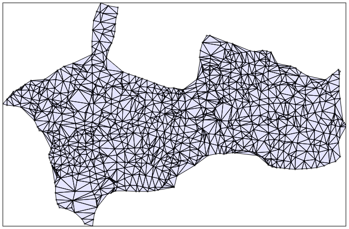
Illustration of each sample processing step of the DtRef method. The triangles conforming to the Delaunay triangulation are shaded in blue:
|
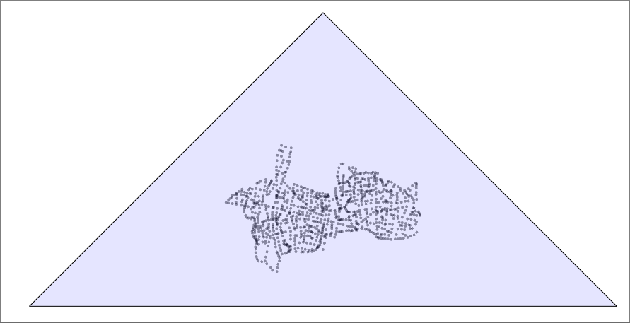
Step 1 Create the super triangle
|
Step 2 Insert the scatter points, conformity is 100%
| ||
|
Step 3 Remove the triangles at the edge of the fictitious envelope
|
Step 4 Remove abnormal triangles on the boundary
|
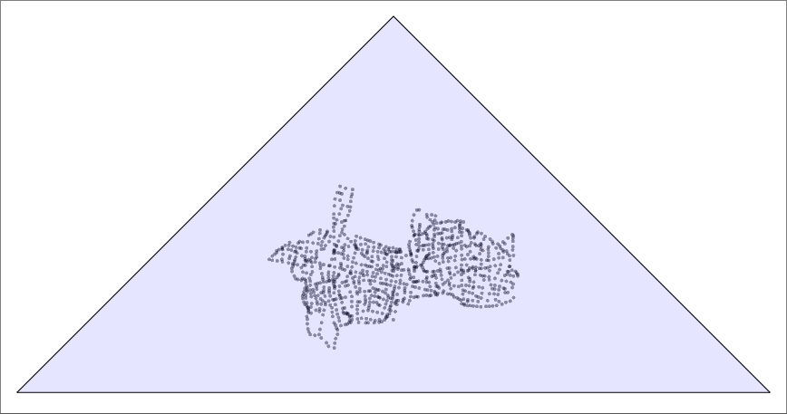
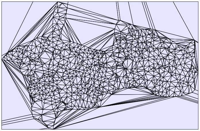
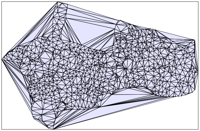
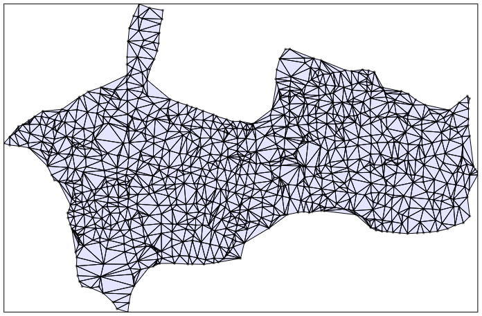
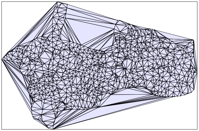
The final step removes boundary triangles whose longest side exceeds a maximum length or whose ratio (height/base length) is below a threshold:
680 meters for our sample.
10% in our case study.
Flip algorithm
The majority of Delaunay triangulation generation algorithms rely on the "Flip" principle that is:
Transforming a triangulation through successive iterations on its non-conforming triangles converges toward conformity.
The algorithms boil down to a two-step construction:
1/ Create the triangulation
2/ Flip adjacent triangles that do not meet the Delaunay criterion
The DtFlipRef method
The "flip principle" is applied to the DtRef method by eliminating the maintenance of Delaunay conformity during each point insertion, replacing it with iterations performed after all points have been inserted.
The method described below is referred to as DtFlipRef in the remainder of the document. It is a simplified version of the DtRef method with the Flip principle.
The most immediate method for creating the triangulation of a point set is to construct the "super triangle", and then to insert the points of the set into it.
Step (1) becomes:
1/ Create the triangulation:
   1.1 Create the super triangle
   1.2 Insert the scatter points
We conclude with the same steps (3 and 4) of the Bowyer–Watson algorithm for removing unnecessary triangles.
The algorithm of the DtFlipRef method can be summarized as follows:
1/ Create the triangulation:
   1.1 Create the super triangle
   1.2 Insert the scatter points
2/ Flip adjacent triangles that do not meet the Delaunay criterion
3/ Remove the triangles at the edge of the fictitious envelope
4/ Remove abnormal triangles on the boundary
Point insertion step (1.2) is performed using nested loops with O(n²) complexity, due to the search for the insertion triangle, which sequentially traverses the created triangles:
1.2 Insert the scatter points
    For each point (p):
    - find the triangle (t) containing point (p)
    - split triangle (t) into three at point (p)
    End loop
After insertion, the percentage of triangles satisfying the Delaunay criterion is recorded in order to compare the methods.
Insert process including edge cases
The detailed insertion Flip insert step (1.2) with edge cases is:
1.2 Insert the scatter points
    For each point (p):
      For each triangle (t)
        - evaluate the state of point (p) for trianle(t):
          - case near vertex:
             - exclude point (p)
             - next point (p)
          - case near segment and near angular sector:
            - set point (p) aside
            - next point (p)
          - case "inside":
            - split triangle (t) into three at point (p)
            - next point (p)
      End of loop (t)
    End of loop (p)
"Near segment and near angular sector" points are set aside for processing after the insertion phase.
Flipping triangles
The Flipping step (2) is performed through successive iterations over the set of triangles while processing the points that were set aside:
2/ Flip adjacent triangles that do not meet the Delaunay criterion
   Do:
      2.1/ Process non-compliant triangles:
           For each triangle (t) in the triangulation:
           - If non-conforming flip the triangle (t) and its relevant adjacent triangle
           End of loop (t)
      2.2/ Process the points set aside
   Continue until 100% conformity is reached
The status of the set-aside points is redetermined when the triangles are transformed to reduce them to two cases:
"inside" case: to split triangle (t) into three at point (p).
"near segment" case: to insert the point onto the segment.
The detailed process of the points set aside is:
2.2/ Process the points set aside
     For each point(p) set aside:
      For each triangle (t):
      - evaluate the status of point (p)
      - "inside" case: split triangle (t)
      - "near vertex" case: exclude point (p)
      - "near segment" case: insert point(p) on segment
      - "near angular sector" case: set point (p) aside
      End of loop (t)
     End of loop (p)
Sample processing
Illustration of each sample processing step of the DtFlipRef method.
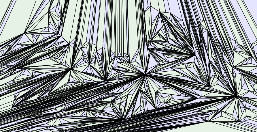
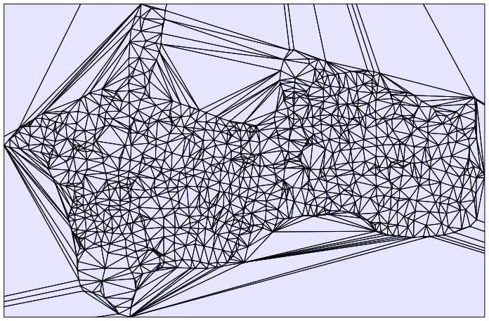
Triangles that do not conform to the Delaunay triangulation are shaded in green:
|
Step 1.1 Create the super triangle
|
Step 1.2 Insert the scatter points, conformity is 40%
| ||
|
Step 2 Flip adjacent triangles that do not meet the Delaunay criterion
|
Step 3 Remove the triangles at the edge of the fictitious envelope
| ||
|
Step 4 Remove abnormal triangles on the boundary
|
DtRef and DtFlipRef metrics for the test dataset
Here is the table of metrics produced by the DtRef and DtFlipRef methods using the test set (981 points).
| Method | Ms | Kb | C. | Objects | Triangle | C. % | Distance | Axis | P. status | Circle | Insert | Split | Shift | Sc. | N. v | N. s | Σ op | Σ pt | B. p | Ratio |
| DtRef | 113 | 265 | 5 | 6,898 | 1,963 | 100 | 5 | 1,547 | 476 | 8 | 981 | 2,928 | 2,038 | 2,077 | 276 | 1 | ||||
| DtFlipRef | 60 | 265 | 5 | 6,898 | 1,963 | 40 | 5 | 1,412 | 441 | 6 | 981 | 3,447 | 9 | 1,867 | 1,903 | 276 | 1 |
Metrics N. v and N. s are empty, indicating good dataset quality.
Similarly, the metric Split indicates the absence of collinear points.
Therefore, this dataset does not allow for testing edge cases.
Comparative analysis of the DtRef and DtFlipRef methods
Both methods yield similar metrics:
The significant difference lies in the number of permutations (Shift), which is higher for DtFlipRef + 17 % (3,447 to 2,928).
This confirms the advantage of maintaining conformity during each insertion in the Bowyer-Watson algorithm,
compared to enforcing conformity after point insertion via successive iterations, as in the flip algorithm.
However, the DtRef method involves a greater number of operations + 9 % (2038,421 to 1867,104)
and is therefore more computationally intensive in terms of geometric calculations.
The DtFlipRef method iterates through the entire set of triangles 9 times to achieve Delaunay conformity of the triangulation.
Calculating point status (476,463) and handling edge cases add complexity to these methods.
Even though the execution time is relatively short (113 ms),
the metrics regarding the number of operations by point (2,077) reveal the O(n²) complexity of this method.
In fact, these methods area heavily dependent on the distribution of the points. The execution time for this phase can vary significantly depending on the dataset.
These methods are useful for creating and validating the implementation of the fundamental triangulation model (relationships between triangles, point status, split segment, split triangle , shift methods, etc.).
Optimization via tree-based sorting
Insert steps of DtRef and DtFlipRef of the previous method is improved by applying the famous "divide and conquer" principle.
To break the O(n²) complexity and reduce the number of point status, points are distributed among the triangles during the point insertion stage.
Each triangle contains the list of included points and is divided into three by the centroid of that list, which is then redistributed among the three new triangles.
With this sorting of the points, the insertion step becomes independent of their distribution.
The algorithm of the DtRef method with tree-based sorting becomes (egde cases are not represented):
1/ Create the "super triangle"
2/ Insert the scatter points

    Add all points to the "super-triangle"

    For each non-empty triangle(t)
    - calculate the midpoint(pc) of the list of included points of triangle(t)
    - split triangle (t) into three at point (pc)
    - distribute the list of included points among the 3 triangles, excluding the central point(pc)
    // Keep Delaunay's conformity
    - As long as there is a non-conforming triangle (ts) around vertex (p):
       - flip the triangle (ts) and its relevant adjacent triangle
    - End of loop (ts)
    Continue as long as there is a non-empty triangle(t)

3/ Remove the triangles at the edge of the fictitious envelope
4/ Remove abnormal triangles on the boundary
This method is referred to as DtRefTree in the remainder of the document.
The algorithm of DtFlipRef method with tree-based sorting becomes (egde cases are not represented):
1/ Create the triangulation:
   1.1 Create the super triangle
   1.2 Insert the scatter points

    Add all points to the "super-triangle"

    For each non-empty triangle(t)
    - calculate the midpoint(pc) of the list of included points of triangle(t)
    - split triangle(t) into three at point(pc)
    - distribute the list of included points among the 3 triangles, excluding the central point(pc)
    Continue as long as there is a non-empty triangle(t)

2/ Flip adjacent triangles that do not meet the Delaunay criterion
3/ Remove the triangles at the edge of the fictitious envelope
4/ Remove abnormal triangles on the boundary
This method is referred to as DtFlipRefTree in the remainder of the document.
The process of finding the triangle for a point is identical to the previous one including edge cases:
Points with "near vertex" status are excluded.
Those classified as "near segment" or "near angular sector" are set aside for processing in step (2) of the triangle transformation.
Triangle subdivision
Sorting orders the points and subdivides the triangles by depth, as shown in the illustrations below for the two methods:
|
DtRefTree division of triangles after one iteration |
DtFlipRefTree division of triangles after one iteration | ||
|
DtRefTree division of triangles after two iterations |
DtFlipRefTree division of triangles after two iterations |
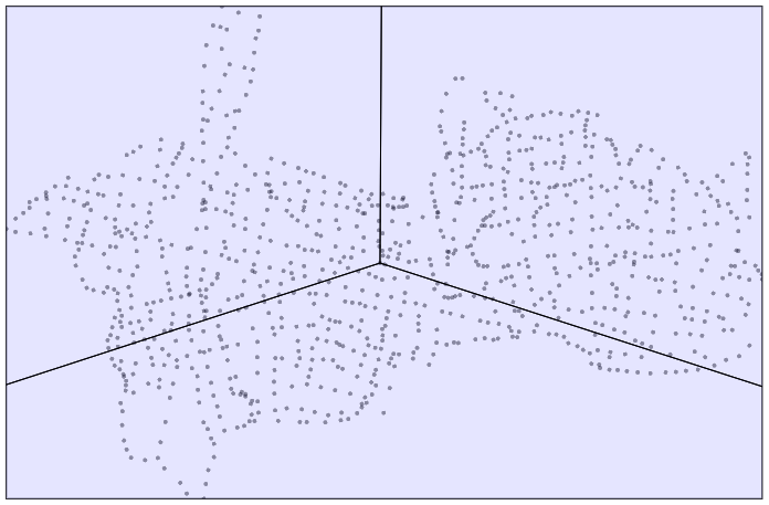
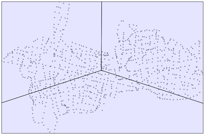
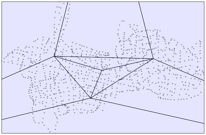
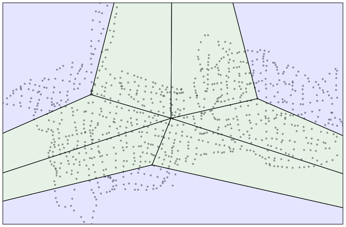
Triangles that do not meet the Delaunay criterion are light green.
Parallel processing
These two methods pave the way for parallelizing the triangulation calculation.
For instance, one can limit the depth of triangle subdivision:
Treat each triangle and its interior points as an independent triangulation to be constructed,.
Then merge them to form the final triangulation.
Merging the triangles requires ensuring the alignment of adjacent triangles along their boundaries.
You can find publications on the "divide and conquer" principle for computing a Delaunay triangulation, such as this one:
DeWall: A fast divide and conquer Delaunay triangulation algorithm.
DtRefTree and DtFlipRefTree metrics for the test dataset
Updating the metrics table with the two new methods DtRefTree and DtFlipRefTree:
| Method | Ms | Kb | C. | Objects | Triangle | C. % | Distance | Axis | P. status | Circle | Insert | Split | Shift | Sc. | N. v | N. s | Σ op | Σ pt | B. p | Ratio |
| DtRef | 113 | 265 | 5 | 6,898 | 1,963 | 100 | 5 | 1,547 | 476 | 8 | 981 | 2,928 | 2,038 | 2,077 | 276 | 1 | ||||
| DtFlipRef | 60 | 265 | 5 | 6,898 | 1,963 | 40 | 5 | 1,412 | 441 | 6 | 981 | 3,447 | 9 | 1,867 | 1,903 | 276 | 1 | |||
| DtRefTree | 22 | 310 | 6 | 9,773 | 1,963 | 100 | 54 | 165 | 27 | 8 | 981 | 2,669 | 1 | 256 | 261 | 323 | 8 | |||
| DtFlipRefTree | 10 | 288 | 6 | 8,393 | 1,963 | 38 | 27 | 103 | 13 | 5 | 981 | 2,936 | 8 | 149 | 152 | 301 | 14 |
Comparative analysis of the DtRefTree and DtFlipRefTree methods
The point insertion steps of DtRefTree and DtFlipRefTree becomes independent of their distribution.
Sorting the points yields an immediate gain:
The number of point status is divided by :
17 and 33 for DtRefTree and DtFlipRefTree methods.
The number of operations is divided by:
8 and 12 for DtRefTree and DtFlipRefTree methods.
Furthermore, the same difference as before is observed between the two methods, just as with the DtRef and DtFlipRef methods:
The number of permutations (Shift) being higher for DtFlipRefTree + 10 % (2,936 to 2,669).
The DtRefTree method still involves a greater number of operations + 71 % (256,630 to 149,796).
Algorithm with convex hull
The "super-triangle" is replaced by a triangulation based on the convex hull of the points.
Benefits are:
No more notional points.
No more reallocation; the method applies directly to the scatter points.
After calculating the convex hull, the triangulation is initialized by determining the point closest to its centroid, and successive triangles are constructed from this center to each side of the boundary.
The initial triangulation is transformed using the "flip principle" to become Delaunay-compliant.
Based on the same principles as the previous methods, two new methods are defined.
The DtCvxTree method, which uses depth-based sorting of points on triangles and transforms non-conforming triangles upon each point insertion.
The DtFlipCvxTree method, which uses depth-based point sorting on triangles and the "flip principle" at the end of insertion.
By analogy with the algorithm of the DtRefTree method, that of the method DtCvxTree becomes (egde cases are not represented):
1/ Create the initial triangulation based on the convex hull and conforming Delaunay.
2/ Insert the scatter points

    - Distribute the points across the triangles

    For each non-empty triangle(t)
    - calculate the midpoint(pc) of the list of included points of triangle(t)
    - split triangle (t) into three at point (pc)
    - distribute the list of included points among the 3 triangles, excluding the central point(pc)
    // Keep Delaunay's conformity
    - As long as there is a non-conforming triangle (ts) around vertex (p):
       - flip the triangle (ts) and its relevant adjacent triangle
    - End of loop (ts)
    Continue as long as there is a non-empty triangle(t)

3/ Remove the triangles at the edge of the fictitious envelope
4/ Remove abnormal triangles on the boundary
Similarly, for the DtFlipCvxTree method, by analogy with the algorithm of the DtFlipRefTree, the algorithm becomes (edge cases are not shown):
1/ Create the triangulation:
   1.1 Create the initial triangulation based on the convex hull and conforming Delaunay.
   1.2 Insert the scatter points

    - Distribute the points across the triangles

    For each non-empty triangle(t)
    - calculate the midpoint(pc) of the list of included points of triangle(t)
    - split triangle(t) into three at point(pc)
    - distribute the list of included points among the 3 triangles, excluding the central point(pc)
    Continue as long as there is a non-empty triangle(t)

2/ Flip adjacent triangles that do not meet the Delaunay criterion
3/ Remove the triangles at the edge of the fictitious envelope
4/ Remove abnormal triangles on the boundary
Convex hull precision
The convex hull is calculated at the same resolution as the precision and filters out points close to its vertices ("near vertex" status).Triangle subdivision with convex hull
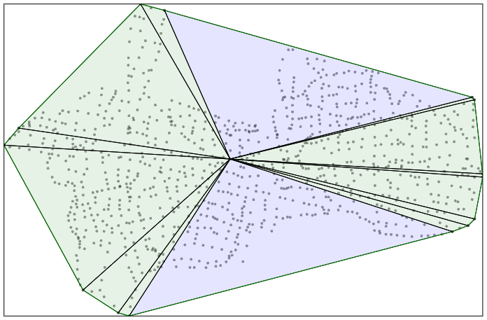
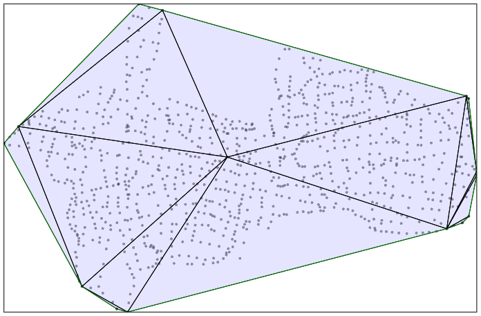
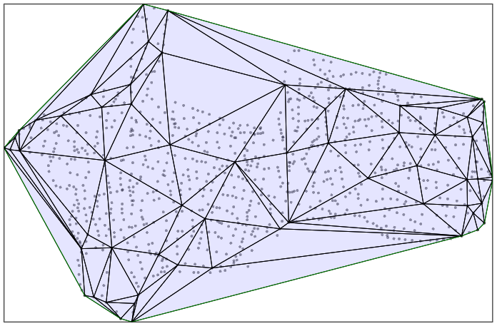
The initial triangulation created with the convex hull comprises 14 triangles.
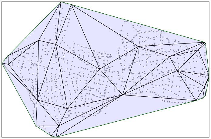
While the previous method starts with only one triangle, this one uses a finer initial triangulation with 14 triangles and conforms more closely to the perimeter of the point set.
The subdivision of the triangles is more precise, as illustrated by the figures below:
|
Triangulation calculated on the convex hull |
Delaunay conformal triangulation | ||
|
Division of triangles after one iteration |
Division of triangles after two iterations |
DtCvxTree and DtFlipCvxTree metrics for the test dataset
The convex hull is calculated in a process (Cvx) separate from the triangulation calculation.
The "Σ ms" column displays the total duration of the method.
Updating the metrics table with the two new methods DtCvxTree and DtFlipCvxTree:
| Method | Ms | Σ ms | Kb | C. | Objects | Triangle | C. % | Distance | Axis | P. status | Circle | Insert | Split | Shift | Sc. | N. v | N. s | Σ op | Σ pt | B. p | Ratio |
| Cvx | 1 | 1 | 0.71 | 3 | 22 | .003 | .049 | .052 | 0.74 | ||||||||||||
| DtRef | 113 | 113 | 265 | 5 | 6,898 | 1,963 | 100 | 5 | 1,547 | 476 | 8 | 981 | 2,928 | 2,038 | 2,077 | 276 | 1 | ||||
| DtFlipRef | 60 | 60 | 265 | 5 | 6,898 | 1,963 | 40 | 5 | 1,412 | 441 | 6 | 981 | 3,447 | 9 | 1,867 | 1,903 | 276 | 1 | |||
| DtRefTree | 22 | 22 | 310 | 6 | 9,773 | 1,963 | 100 | 54 | 165 | 27 | 8 | 981 | 2,669 | 1 | 256 | 261 | 323 | 8 | |||
| DtFlipRefTree | 10 | 10 | 288 | 6 | 8,393 | 1,963 | 38 | 27 | 103 | 13 | 5 | 981 | 2,936 | 8 | 149 | 152 | 301 | 14 | |||
| DtCvxTree | 37 | 45 | 281 | 9 | 8,702 | 1,946 | 100 | 53 | 189 | 31 | 8 | 966 | 2,628 | 283 | 288 | 293 | 7 | ||||
| DtFlipCvxTree | 12 | 20 | 260 | 9 | 7,363 | 1,946 | 39 | 24 | 131 | 21 | 6 | 966 | 3,129 | 8 | 2 | 183 | 187 | 293 | 11 |
Comparative analysis of the DtCvxTree and DtFlipCvxTree methods
Observations on metrics:
Calculating the convex hull is very fast (1 ms) and has no impact on the total computation time.
The indicators of DtCvxTree and DtFlipCvxTree remain equivalent to those of the previous methods DtRefTree and DtFlipRefTree respectively.
The advantage of the Bowyer-Watson algorithm (DtCvxTree method) is preserved with a reduced number - 16 % (from 2,628 to 3,129) of transformations (Shift).
The DtCvxTree method still involves a greater number of operations + 35 % (from 283,157 to 183,886).
Reduces the number of unnecessary triangles along the boundary.
Calculation of a convex hull
The calculation is performed at a specific resolution, and the algorithm eliminates points that coincide with the selected vertices.
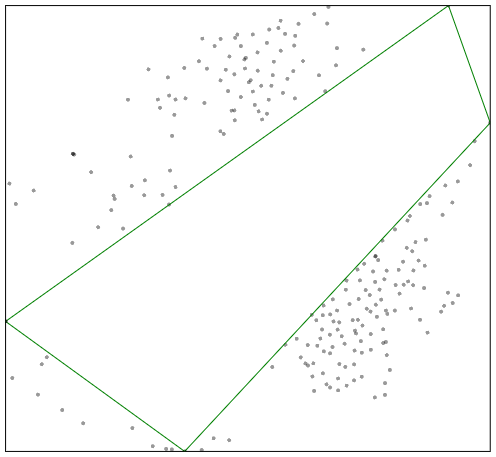
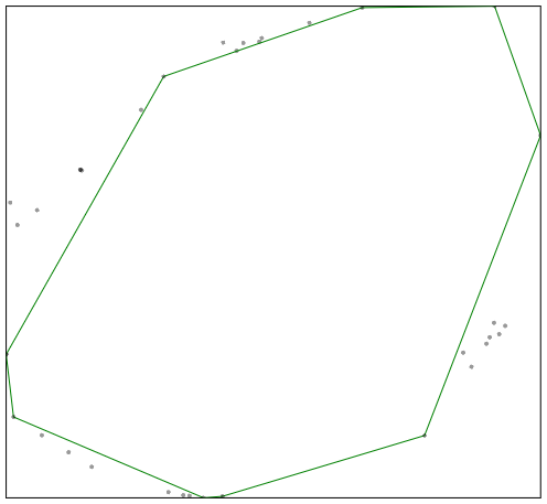
Here is a simple and efficient algorithm for calculating the convex hull of a set of points that uses the "divide and conquer" principle:
 Initialize the convex hull with the extreme points (x_min, y_max, x_max, y_min).
 Distribute each point located outside the convex hull onto its corresponding projected segment.
 For each non-empty segment (s):
 - Determine the highest point
 - Split the segment (s) at that point
 - Redistribute the points of (s) across the two segments
 End loop (s)
The complexity of the algorithm is O(n log n).
|
The convex hull of the extreme points and its exterior points |
Convex after one iteration |
Convex ring algorithm
This method offers an original approach using a classification of points by concentric rings to carry out the first step of creating the triangulation.
The CvxSurface structure
To achieve this, the convex hull calculation is used to accumulate within a structure (named CvxSurface) all the hulls of the points, proceeding from the outside toward the center; each hull is determined using the points located inside the preceding one. The final contour may consist of three or more points, or it may be flattened into two points or even a single point.
The calculation method for the CvxSurface structure is as follows:
Calculate the convex hull (cvx1) of the set of points
While (cvx1) contains points
 Calculate the convex hull (cvx2) of the points inside (cvx1)
 Continue with (cvx2), which becomes (cvx1)
The CvxRing structure
A second structure (named CvxRing) is derived from the CvxSurface and consists of adjacent concentric rings delimited by two successive convex hulls (an inner one and an outer one), plus a final solid ring with no inner contour.
|
The structure CvxSurface classifies the 981 points into 50 contours. |
The CvxRing structure is composed of 49 rings and a solid last one. |
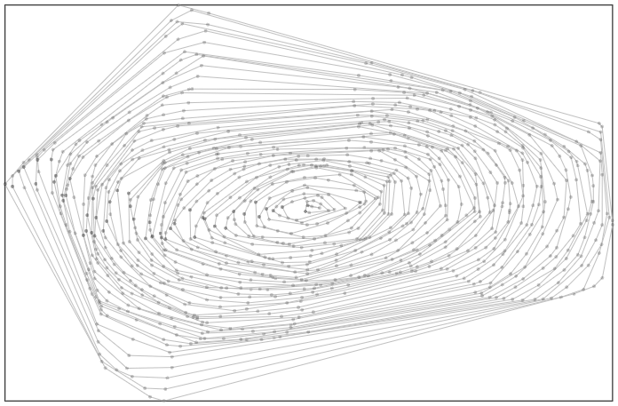
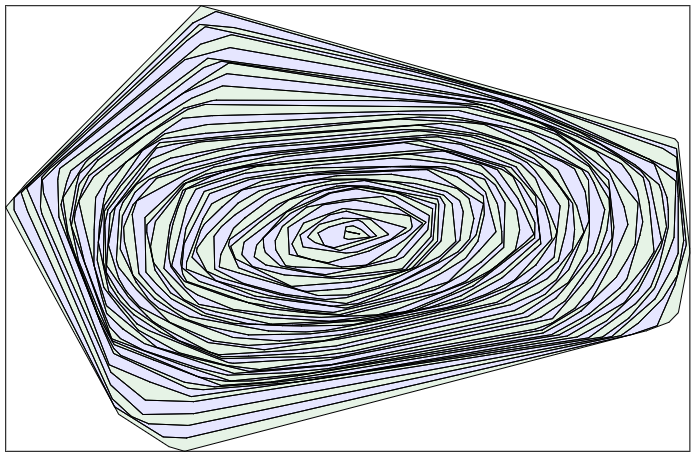
The rings (represented here by alternating shades of green and light blue) cover the space and pass through every point without intersecting.
Triangulation cursor
|
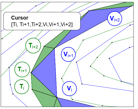
The area of each ring, bounded by its two boundaries, can be triangulated using triangles adjacent to either the outer (green) boundary or the inner (blue) boundary (Triangulation of rings).
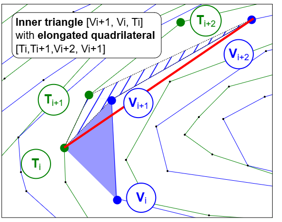
To triangulate a ring, a cursor is used on three successive points of its outer (T
The cursor defines a quadrilateral [T
The first two vertices define either the triangle adjacent to the outer contour [T |
|
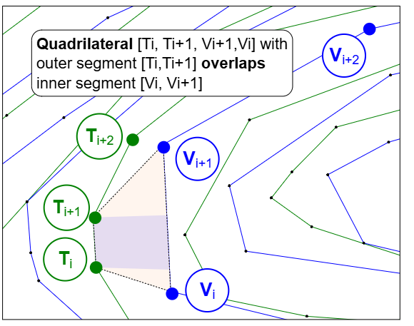
Optimal triangle
|
As for the third vertices T
|
|
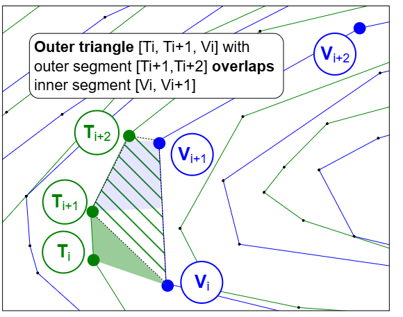
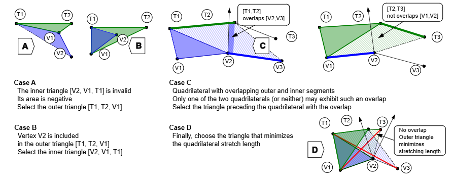
Choice of triangle
The choice of triangle is made based on the analysis of the vertices (4 cases):
|
|
Triangulation of the Cvx Ring structure
The CvxRing structure thus allows the triangulation to be partitioned ring by ring:
Each ring constitutes a triangulation.
The triangles located on the outer edge of a ring are all adjacent, along their longest side, to the triangles on the inner edge of the preceding ring.
The relationships between the triangles of two consecutive rings are easy to establish.
The triangulation of each ring primarily produces flat triangles, however:
The transformation of triangles converges rapidly, ring by ring.
Starting with the application of the base-max criterion to the inner boundary of eaf ring.
The transformation of the triangles is carried out in five steps:
4/ Transform the triangles on each ring
   For each ring (r) other than the last one:
   - Flip triangles that do not meet the base-max criterion on the inner boundary of the ring (r)
   End of loop (r)
   For each ring (r) other than the last one:
   - Flip triangles that do not meet the Delaunay criterion on the inner boundary of the ring (r)
   End of loop (r)
   For each ring (r):
   - Flip triangles that do not meet the Delaunay criterion on the outer boundary of the ring (r)
   End of loop (r)
   - Flip triangles that do not meet the Delaunay criterion on the last ring
Following the calculation of the CvxSurface structure, the calculation method for the CvxRing structure is as follows:
Compute the (CvxRing) structure from the CvxSurface structure:
1/ Create the rings for each contour
2/ Triangulate each ring
3/ Establish relationships between the triangles at the edges of each ring
4/ Transform the triangles on each ring
Several steps can be parallelized:
Step 2, Triangulate each ring can be processed in parallel ring by ring.
It is also possible to transform the ring triangles at this stage if processed in parallel.
This makes it possible to reduce the number of transformations to be handled after the links between rings are created.
Step 3, Establishing the relationships between rings can be handled in parallel, group by group of adjacent rings.
|
Triangulate each ring |
Transform triangles on each ring, conformity is 100% |
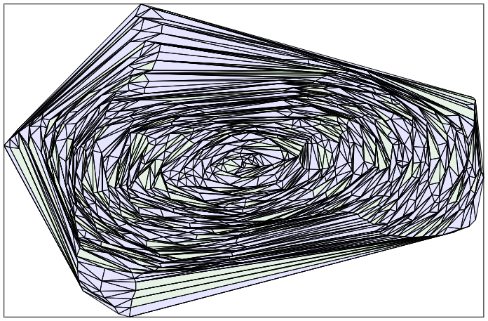
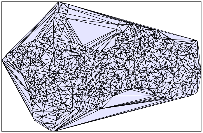
The algorithm with the CvxRing structure
Once the CvxRing structure has been calculated, the triangulation can be formed by accumulating the triangles from the rings.
The new algorithm can be summarized as follows:
0/ Calculate the two structures CvxSurface and CvxRing (which can be processed during a separate upstream step)
1/ Create the triangulation by accumulating the rings (after this step, the triangulation is Delaunay compliant)
2/ Remove abnormal triangles on the boundary
Edge cases
Edge cases are naturally handled by the method that does not require calculating the point status:
The computation of convex hulls eliminates nearby points ("near vertex").
The CvxRing triangulation is performed without insertions, thus eliminating the need to analyze edge cases "near segment", "near angular sector"), which are resolved by flipping maximal bases.
DtCvxRing metrics for the test dataset
Updating the metrics table with the new method DtCvxRing with calculations of the CvxSurface and CvxRing structures prior to the triangulation calculation:
| Method | Ms | Σ ms | Kb | C. | Objects | Triangle | C. % | Distance | Axis | P. status | Circle | Insert | Split | Shift | Sc. | N. v | N. s | Σ op | Σ pt | B. p | Ratio |
| Cvx | 1 | 1 | 0.71 | 3 | 22 | .003 | .049 | .052 | 0.74 | ||||||||||||
| CvxSurface | 42 | 42 | 49 | 5 | 1,386 | .352 | 3 | 4 | 4 | 51 | |||||||||||
| CvxRing | 34 | 76 | 303 | 10 | 6,783 | 1,946 | .548 | 39 | 4 | 2,291 | 48 | 49 | 316 | ||||||||
| DtRef | 113 | 113 | 265 | 5 | 6,898 | 1,963 | 100 | 5 | 1,547 | 476 | 8 | 981 | 2,928 | 2,038 | 2,077 | 276 | 1 | ||||
| DtFlipRef | 60 | 60 | 265 | 5 | 6,898 | 1,963 | 40 | 5 | 1,412 | 441 | 6 | 981 | 3,447 | 9 | 1,867 | 1,903 | 276 | 1 | |||
| DtRefTree | 22 | 22 | 310 | 6 | 9,773 | 1,963 | 100 | 54 | 165 | 27 | 8 | 981 | 2,669 | 1 | 256 | 261 | 323 | 8 | |||
| DtFlipRefTree | 10 | 10 | 288 | 6 | 8,393 | 1,963 | 38 | 27 | 103 | 13 | 5 | 981 | 2,936 | 8 | 149 | 152 | 301 | 14 | |||
| DtCvxTree | 37 | 45 | 281 | 9 | 8,702 | 1,946 | 100 | 53 | 189 | 31 | 8 | 966 | 2,628 | 283 | 288 | 293 | 7 | ||||
| DtFlipCvxTree | 12 | 20 | 260 | 9 | 7,363 | 1,946 | 39 | 24 | 131 | 21 | 6 | 966 | 3,129 | 8 | 2 | 183 | 187 | 293 | 11 | ||
| DtCvxRing | 4 | 80 | 318 | 12 | 6,800 | 1,946 | 100 | 35 | 2,291 | 84 | 86 | 332 | 24 |
Analysis of the DtCvxRing method
Observations on metrics:
The execution of the DtCvxRing method is very fast (4 ms) because it simply involves importing the ring triangles into its triangulation and then removing the anomalous triangles located on the boundary.
The conformity of the triangles after creating the CvxRing structure is 100%.
The number of transformations (Shift) performed by CvxRing is low (2,291 compared to 2,928 for the DtRef method) representing a 21 % reduction.
Triangle transformations are performed without traversing the entire triangulation, but solely on the boundaries of the rings.
The number of operations per point (Σ pt) of DtCvxRing is also the lowest (86 compared to 2,077 for the DtRef method) representing a 95 % reduction or a ratio of 1/24.
While the amount of memory in bytes per point (332 compared to 276 for the DtRef method) is the greatest, representing a 20 % increase.
In conclusion:
The method is more complex to implement and consumes more memory 318/265 Kb.
The method's logic is distributed across three components (CvxSurface, CvxRing, DtCvxRing) rather than concentrated in a single monolithic component.
The scalability of the method, achieved by decomposing the set of points into concentric rings, combined with its parallelizability, enables it to handle larger volumes.
Evaluation with other datasets
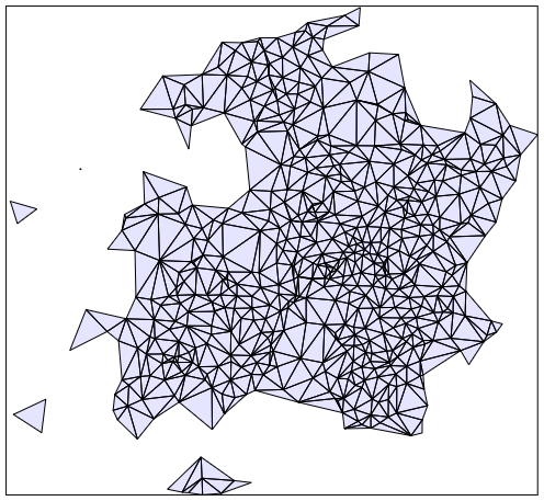
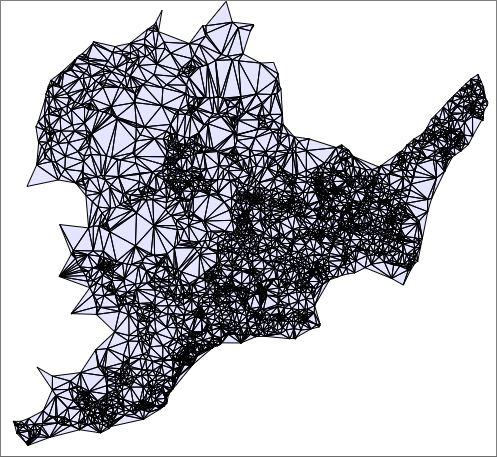
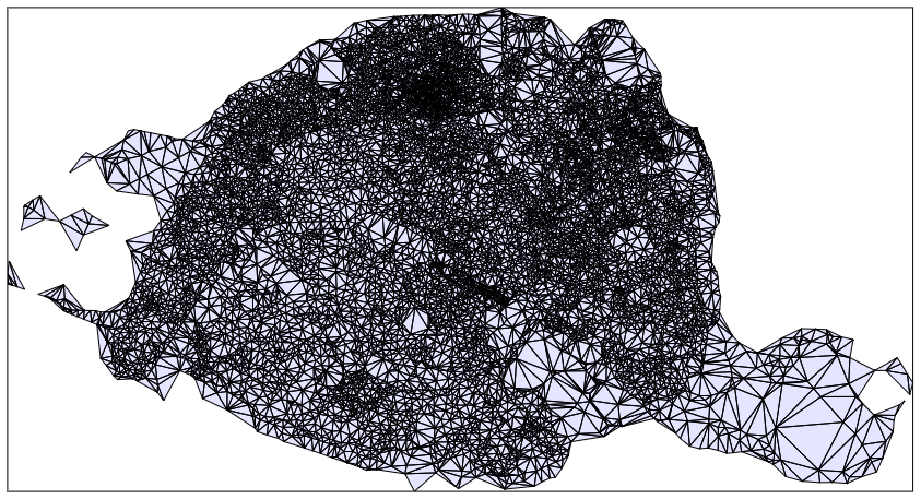
To complement the evaluation of the methods, three additional datasets, all derived from topographic surveys, are used.
|
569 points |
3,839 points |
9,811 points |
The second dataset
The second dataset is a topographic survey with 569 points.
| Method | Ms | Σ ms | Kb | C. | Objects | Triangle | C. % | Distance | Axis | P. status | Circle | Insert | Split | Shift | Sc. | N. v | N. s | Σ op | Σ pt | B. p | Ratio |
| Cvx | 7 | 7 | 0.83 | 3 | 26 | .003 | .065 | .068 | 1 | ||||||||||||
| CvxSurface | 23 | 23 | 31 | 5 | 870 | .272 | 2 | 2 | 4 | 55 | |||||||||||
| CvxRing | 23 | 46 | 184 | 10 | 4,159 | 1,118 | .332 | 19 | 2 | 1,134 | 24 | 43 | 331 | ||||||||
| DtRef | 58 | 58 | 154 | 5 | 4,014 | 1,139 | 100 | 3 | 585 | 173 | 4 | 569 | 1,599 | 767 | 1,347 | 277 | 1 | ||||
| DtFlipRef | 34 | 34 | 154 | 5 | 4,014 | 1,139 | 38 | 3 | 511 | 153 | 3 | 569 | 2,034 | 8 | 672 | 1,181 | 277 | 1 | |||
| DtRefTree | 16 | 16 | 180 | 6 | 5,675 | 1,139 | 100 | 29 | 90 | 14 | 4 | 569 | 1,514 | 138 | 243 | 324 | 6 | ||||
| DtFlipRefTree | 10 | 10 | 167 | 6 | 4,894 | 1,139 | 39 | 15 | 56 | 7 | 3 | 569 | 1,571 | 6 | 82 | 144 | 302 | 9 | |||
| DtCvxTree | 21 | 33 | 161 | 9 | 4,998 | 1,118 | 100 | 29 | 106 | 17 | 4 | 550 | 1,473 | 158 | 279 | 291 | 5 | ||||
| DtFlipCvxTree | 13 | 25 | 149 | 9 | 4,235 | 1,118 | 39 | 12 | 65 | 9 | 3 | 550 | 1,645 | 8 | 90 | 158 | 269 | 9 | |||
| DtCvxRing | 3 | 49 | 192 | 12 | 4,176 | 1,118 | 100 | 20 | 1,134 | 44 | 78 | 347 | 17 |
The third dataset
The third dataset contains 3,839 points (1 of which are excluded due to their proximity to another point).
| Method | Ms | Σ ms | Kb | C. | Objects | Triangle | C. % | Distance | Axis | P. status | Circle | Insert | Split | Shift | Sc. | N. v | N. s | Σ op | Σ pt | B. p | Ratio |
| Cvx | 11 | 11 | 0.71 | 3 | 22 | .003 | .049 | .052 | 0.18 | ||||||||||||
| CvxSurface | 176 | 176 | 177 | 5 | 4,987 | 1 | 14 | 1 | 16 | 4 | 47 | ||||||||||
| CvxRing | 63 | 239 | 1,127 | 10 | 24,961 | 7,660 | 2 | 202 | 21 | 11,675 | 242 | 63 | 300 | ||||||||
| DtRef | 1,053 | 1,053 | 1,035 | 5 | 26,902 | 7,677 | 100 | 23 | 22,086 | 7,147 | 34 | 3,832 | 12 | 11,338 | 1 | 13 | 29,291 | 7,629 | 276 | 1 | |
| DtFlipRef | 848 | 848 | 1,035 | 5 | 26,900 | 7,677 | 37 | 23 | 20,442 | 6,695 | 26 | 3,838 | 14,372 | 9 | 1 | 6 | 27,187 | 7,081 | 276 | 1 | |
| DtRefTree | 63 | 63 | 1,211 | 6 | 38,143 | 7,677 | 100 | 270 | 1,152 | 202 | 32 | 3,830 | 16 | 10,502 | 1 | 24 | 1,657 | 431 | 323 | 18 | |
| DtFlipRefTree | 50 | 50 | 1,126 | 6 | 32,763 | 7,677 | 38 | 124 | 882 | 189 | 23 | 3,832 | 12 | 11,871 | 9 | 1 | 20 | 1,219 | 317 | 300 | 24 |
| DtCvxTree | 143 | 154 | 1,103 | 9 | 34,202 | 7,660 | 100 | 288 | 1,520 | 291 | 32 | 3,813 | 20 | 10,414 | 1 | 29 | 2,133 | 555 | 294 | 14 | |
| DtFlipCvxTree | 49 | 60 | 1,020 | 9 | 28,871 | 7,660 | 39 | 115 | 697 | 132 | 25 | 3,821 | 4 | 13,569 | 10 | 1 | 12 | 970 | 252 | 272 | 30 |
| DtCvxRing | 10 | 249 | 1,186 | 12 | 24,978 | 7,660 | 100 | 127 | 11,675 | 370 | 96 | 316 | 79 |
The fourth dataset
The fourth dataset contains 9,811 points (1 of which are excluded due to their proximity to another point).
| Method | Ms | Σ ms | Kb | C. | Objects | Triangle | C. % | Distance | Axis | P. status | Circle | Insert | Split | Shift | Sc. | N. v | N. s | Σ op | Σ pt | B. p | Ratio |
| Cvx | 19 | 19 | 1 | 3 | 33 | .003 | .093 | .096 | 0.11 | ||||||||||||
| CvxSurface | 323 | 323 | 412 | 5 | 11,623 | 1 | 38 | 1 | 40 | 4 | 43 | ||||||||||
| CvxRing | 95 | 418 | 2,701 | 10 | 58,031 | 19,593 | 5 | 545 | 56 | 31,936 | 647 | 65 | 281 | ||||||||
| DtRef | 6,359 | 6,359 | 2,644 | 5 | 68,706 | 19,621 | 100 | 59 | 140,658 | 46,233 | 87 | 9,800 | 20 | 28,991 | 1 | 24 | 187,038 | 19,064 | 276 | 1 | |
| DtFlipRef | 5,263 | 5,263 | 2,644 | 5 | 68,706 | 19,621 | 39 | 59 | 134,492 | 44,464 | 72 | 9,804 | 12 | 40,983 | 10 | 1 | 29 | 179,088 | 18,253 | 276 | 1 |
| DtRefTree | 284 | 284 | 3,097 | 6 | 97,675 | 19,621 | 100 | 805 | 5,269 | 1,048 | 83 | 9,792 | 36 | 26,831 | 1 | 57 | 7,206 | 734 | 323 | 26 | |
| DtFlipRefTree | 141 | 141 | 2,878 | 6 | 83,650 | 19,621 | 39 | 338 | 3,126 | 687 | 66 | 9,796 | 28 | 36,045 | 10 | 1 | 45 | 4,218 | 430 | 300 | 44 |
| DtCvxTree | 514 | 523 | 2,828 | 9 | 87,922 | 19,593 | 100 | 815 | 5,802 | 1,126 | 83 | 9,764 | 40 | 27,062 | 1 | 64 | 7,829 | 797 | 295 | 24 | |
| DtFlipCvxTree | 253 | 262 | 2,607 | 9 | 73,765 | 19,593 | 39 | 307 | 3,479 | 806 | 68 | 9,772 | 24 | 37,383 | 10 | 1 | 46 | 4,662 | 475 | 272 | 40 |
| DtCvxRing | 16 | 434 | 2,853 | 12 | 58,048 | 19,593 | 100 | 325 | 31,936 | 972 | 99 | 297 | 193 |
Assessment of method complexity
To evaluate the complexity of the methods, their metrics are analyzed across the four datasets, based on:
The number of operations (Σ op) required to compute the triangulation for each dataset. independently of the language and execution platform.
The number of points of each dataset (
np).
| Method | Number of operations (Σ op) in thousands by dataset | |||
| DtRef | 767 | 2,038 | 29,291 | 187,038 |
| DtFlipRef | 672 | 1,867 | 27,187 | 179,088 |
| DtRefTree | 138 | 256 | 1,657 | 7,206 |
| DtFlipRefTree | 82 | 149 | 1,219 | 4,218 |
| DtCvxTree | 158 | 283 | 2,133 | 7,829 |
| DtFlipCvxTree | 90 | 183 | 970 | 4,662 |
| DtCvxRing | 44 | 84 | 370 | 972 |
Dataset points (np) | 569 | 981 | 3,839 | 9,811 |
Method for evaluating correlation equations for the number of operations
By treating the measurements (Σ op, np) obtained for each method as a series, probabilistic techniques (calculation of standard deviation, variance, and variation) are applied to evaluate the correlation equations.
Subsequently, to evaluate a correlation equation Σ op=f(np), its percentage variation (standard deviation divided by the mean value) is calculated across the five datasets.
A percentage variation of less than 15% is accepted as an indicator of the equation's plausibility.
Evaluation of the complexity of the DtRef method
For the DtRef method, as expected given its O(n²) complexity, we observe that the value 2*(np)² is close to the value Σ op, as shown by the calculation for the last dataset:
2*(np)² = 2*(3,839)² = 29475,842 op = 29291,302.
To confirm this equation for this method and DtFlipRef, we calculate its percentage variation:
| Method | Equation | Variation % |
| DtRef |
Σ op ≈
2.01 * ( np ^ 2.01)
| 8.65 |
| DtFlipRef |
Σ op ≈
2.0 * ( np ^ 2.0)
| 4.37 |
The value of the variation is less than 15%, confirming the equation.
To proceed, we represent this equation on a graph with for each method:
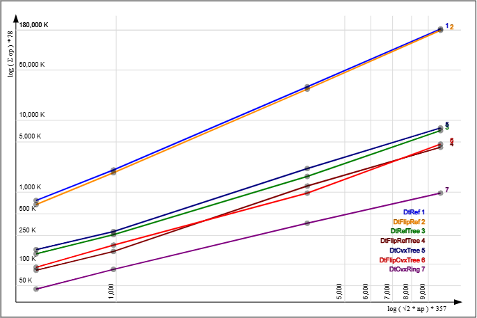 |
It can be seen from the graph that:
The correlation for the DtRef and DtFlipRef methods is confirmed by the alignment of the points on its curve (1).
The curves corresponding to the four methods DtRefTree (3), DtFlipRefTree (4), DtCvxTree (5), DtFlipCvxTree (6) are close to one another, and their points are nearly aligned.
In contrast, the DtCvxRing curve (7) deviates from the previous four, and its points are not aligned.
It is assumed that:
The four methods DtRefTree, DtFlipRefTree, DtCvxTree, DtFlipCvxTree, which are optimizations of DtRef and DtFlipRef, follow the same law with different coefficients.
Whereas DtCvxRing follows a different one.
Complexity evaluation of the DtRefTree, DtFlipRefTree, DtCvxTree and DtFlipCvxTree methods
We generalize the DtRef equation to determine the equations for the other four by calculating:
Its selection of the best correlation for each method leads to the following equations :
| Method | (f) | K(f) | V(f) % | Σ op | Variation % |
| DtRef | 1 | 2.01 | 0.55 |
≈
2.01 * ( np ^ 2.01)
| 8.65 |
| DtFlipRef | 1 | 2.0 | 0.29 |
≈
2.0 * ( np ^ 2.0)
| 4.37 |
| DtRefTree | 6 | 1.39 | 0.58 |
≈
19.41 * ( np ^ 1.39)
| 7.75 |
| DtFlipRefTree | 4 | 1.4 | 0.59 |
≈
11.23 * ( np ^ 1.4)
| 7.05 |
| DtCvxTree | 7 | 1.38 | 0.53 |
≈
23.63 * ( np ^ 1.38)
| 6.46 |
| DtFlipCvxTree | 6 | 1.34 | 0.77 |
≈
17.65 * ( np ^ 1.34)
| 10.84 |
Following this calculation, we observe:
Next, the (Σ op / np^√2) ratio of the equation is determined for the three methods, followed by the variation:
| Method | Equation | Variation % |
| DtRef |
Σ op ≈
2.01 * ( np ^ 2.01)
| 8.65 |
| DtFlipRef |
Σ op ≈
2.0 * ( np ^ 2.0)
| 4.37 |
| DtRefTree |
Σ op ≈
15.79 * ( np ^ √2)
| 8.28 |
| DtFlipRefTree |
Σ op ≈
9.79 * ( np ^ √2)
| 6.86 |
| DtCvxTree |
Σ op ≈
18.19 * ( np ^ √2)
| 7.03 |
| DtFlipCvxTree |
Σ op ≈
10.27 * ( np ^ √2)
| 11.64 |
Complexity evaluation of the DtCvxRing method
For the DtCvxRing method, and in order to confirm the assumed O(n log n) complexity, we evaluate the following ratio R(p):
R(
p) = log( Σ op ) / log(p*np* log(np) ).We are looking for the value of (
p) for which the ratio R(p) is close to 1, with a variation V(p) of less than 1%.
A bisection search on the interval [1, 100] for (p) :
Yields a value of (
p) equal to 11.897, with a variation V(p) of 0.47%.Ultimately, the variation of the correlation equation Σ op ≈ 11.897 *
np* log(np) is 5.83%, confirming the hypothesis of O(n log n) complexity.
Summary of the method complexity assessment
The table below summarizes the correlation equation (Σ op ≈ f(np)), the percentage of variation, and the complexity for each method:
| Method | Equation | Variation % | Complexity |
| DtRef |
Σ op ≈
2.01 * ( np ^ 2.01 )
| 8.65 | O( np² ) |
| DtFlipRef |
Σ op ≈
2.0 * ( np ^ 2.0 )
| 4.37 | O( np² ) |
| DtRefTree |
Σ op ≈
15.79 * ( np ^ √2 )
| 8.28 | O( np^√2 ) |
| DtFlipRefTree |
Σ op ≈
9.79 * ( np ^ √2 )
| 6.86 | O( np^√2 ) |
| DtCvxTree |
Σ op ≈
18.19 * ( np ^ √2 )
| 7.03 | O( np^√2 ) |
| DtFlipCvxTree |
Σ op ≈
10.27 * ( np ^ √2 )
| 11.64 | O( np^√2 ) |
| DtCvxRing |
Σ op ≈ 11.897 * np * log( np )
| 5.83 | O( np*log(np) ) |
To complement this table, the following graph shows:
The curves (y=log(Σop),x=
np) for each method.Along with their correlation equations (gray dashed line).
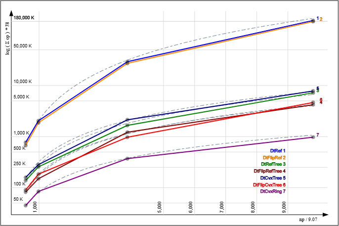 |
A scale factor is applied to each axis to fit the 4:3 ratio.
Evaluating the strengths and weaknesses of the methods
To evaluate the strengths and weaknesses of the methods, we rely on criteria based on metrics.
When weighed against the requirements of the application context, these criteria help guide the choice.
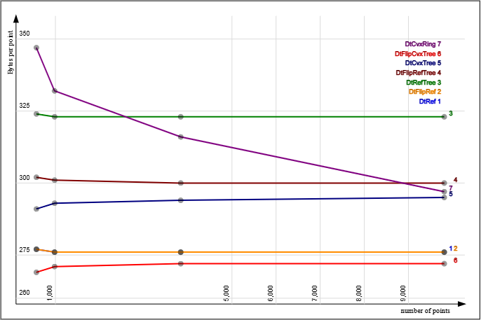
The two metrics, number of operations per point (Σ pt) and number of bytes per point (B. p), are decisive in the evaluation of the methods, as shown by their graphs:
|
Number of operations per point |
Number of bytes per point |
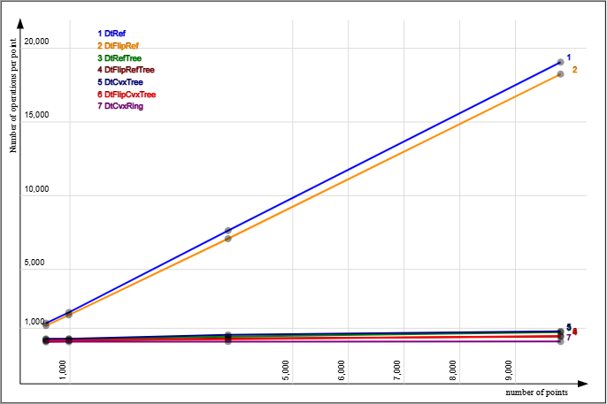
For production deployment, the DtRef and DtFlipRef methods are unacceptable due to their O(n²) complexity, as shown by the graph of the number of operations per point.
The choice therefore falls on the other five methods.
The second graph, showing the number of bytes per point, reveals:
that this value remains practically constant for the four methods other than DtCvxRing
whereas for the latter, it decreases to 297 bytes for the final dataset containing 9,811 points.
We will therefore use the measurements obtained on the final dataset to compare the last five methods.
|
Number of operations per point |
Number of bytes per point |
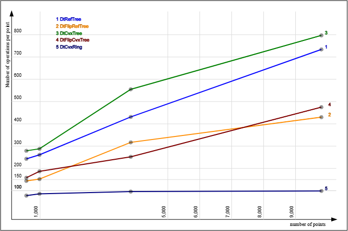
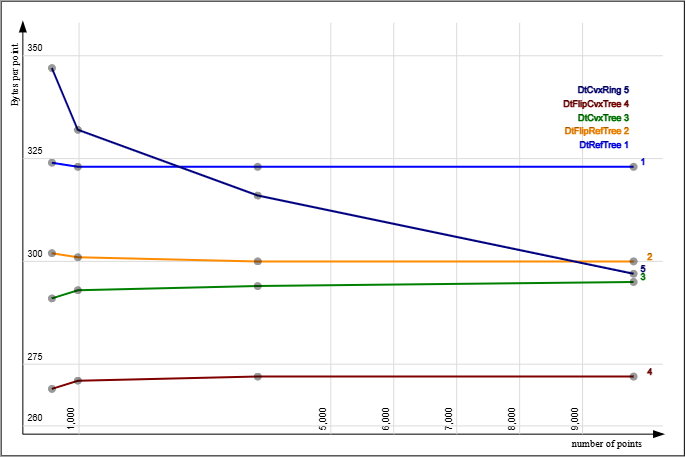
After narrowing the choice down to the five last methods, the graph showing the number of operations per point reveals:
that the metric for the first four methods ranges from 144 to 797,
whereas for the DtCvxRing method, the metric remains close to 100, from 78 to 99,
combined with a byte count per point of 347 to 297,
demonstrating the method's high execution stability.
The evaluation of the methods is based on quantified criteria and design-related criteria.
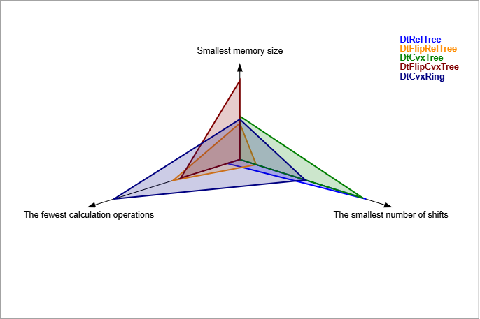
Quantified evaluation criteria
We use the measurements obtained on the final dataset to compare the last five methods.
Each criterion results in a score from 1 to 10.
| Criteria |
|
Evaluation of methods using quantified criteria
|
|
Design criteria
These criteria do not result in a measured score but identify a characteristic classified as a strength.
| Strength / Weakness |
|
Evaluation of methods using design criteria
| Strength / Weakness | DtRefTree | DtFlip.. | DtCvxTree | DtFlip.. | DtCvxRing |
| Flexible design processing | No | No | No | No | Yes |
| Operates on dataset points | No | No | Yes | Yes | Yes |
| Parallel processing | No (1) | No (1) | No (1) | No (1) | Yes |
Complexity O( np*log(np) )
| No | No | No | No | Yes |
(1) Parallelizing depth-first sorting methods is possible, provided the algorithm undergoes significant modifications.
General conclusion
The last five methods can be distinguished as follows:
The group of the two methods (DtRefTree, DtCvxTree) based on the Bowyer-Watson algorithm.
These methods proceed by iteration, without traversing all the triangles.
The second method (DtCvxTree) has two advantages, as it consumes less memory and directly uses the points from the dataset.
The second group of the two methods (DtFlipRefTree, DtFlipCvxTree) that uses the flip pinciple.
The flip principle is simpler to implement than the Bowyer-Watson iteration.
However, these methods involve more shifts than the previous ones.
The second method (DtFlipCvxTree) retains its advantages, just as in the previous group.
And finally, the DtCvxRing method, which is orthogonal to the previous ones.
This last method differs from the others in that:
A concentric ring design, as opposed to the point-injection design of other methods.
And indeed, it does not use complex operations for inserting a point into a triangle or onto a segment.
Is using only the axis tool for all these calculations.
A simple and effective treatment for edge cases.
Stable execution,
evidenced by metrics indicating an operation-per-point count close to 100 (from 78 to 99) and a byte-per-point count approaching 300 (from 347 to 297).
A more flexible design built on 12 classes.
An algorithm complexity of O(
np*log(np) ).Some stages of the processing can be parallelized.
References
Delaunay triangulation
Delaunay, B. (1934). Sur la sphère vide. A la mémoire de Georges Voronoi. Bulletin de l'Académie des Sciences de l'URSS, Class. Sci. Nat.
De Berg, M., Cheong, O., van Kreveld, M., Overmars, M. (2008). Computational Geometry: Algorithms and Applications (3rd ed.). Springer.
Cheng, S. W., Dey, T. K., Shewchuk, J. (2012). Delaunay Mesh Generation. CRC Press.
Bowyer-Watson algorithm
Bowyer, A. (1981). Computing Dirichlet tessellations. The Computer Journal, 24(2), 162-166.
Watson, D. F. (1981). Computing the n-dimensional Delaunay tessellation with applications to Voronoi polytopes. The Computer Journal, 24(2), 167-172.
Lawson's Flip
Lawson, C. L. (1977). Software for C1 surface interpolation. In Mathematical Software III (pp. 161-194). Academic Press.
Edelsbrunner, H., Shah, N. R. (1996). Incremental topological flipping works for regular triangulations. Algorithmica, 15(3), 223-241
Divide and Conquer algoritm
Guibas, L., Stolfi, J. (1985). Primitives for the manipulation of general subdivisions and the computation of Voronoi diagrams. ACM Transactions on Graphics (TOG), 4(2), 74-123.
Shamos, M. I., Hoey, D. (1975). Closest-point problems. In 16th Annual Symposium on Foundations of Computer Science (FOCS) (pp. 151-162). IEEE.
Convex hull of a point set
F. P. Preparata et S. J. Hong. (1977). Convex hulls of finite sets of points in two and three dimensions.
David G. Kirkpatrick et Raimund Seidel. (1986). The Ultimate Planar Convex Hull Algorithm.